Backtesting is the backbone of risk management in futures trading. It helps you understand how a strategy might perform under various market conditions, reducing guesswork and emotional decision-making. By analyzing critical metrics like maximum drawdown, win rate, and profit factor, you can fine-tune your approach to manage risk effectively, especially when pursuing funding from best futures prop firms.
Key Takeaways:
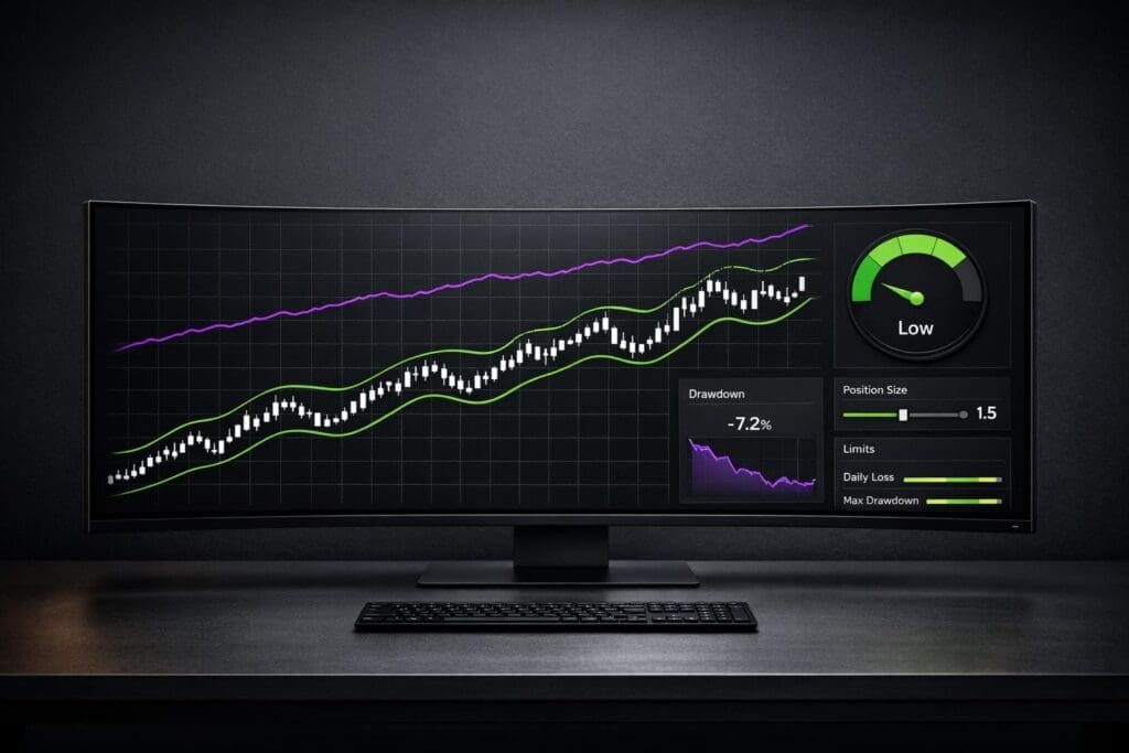
- Maximum Drawdown (MDD): Reveals your worst-case loss. Keep drawdowns under control by halting strategies that approach 70% of your allowed drawdown.
- Risk of Ruin (RoR): Calculate the probability of account failure. Aim for RoR below 5% for retail trading.
- Position Sizing: Use methods like Fixed Fractional (1–2% risk per trade) or the Kelly Criterion to balance growth and risk.
- Dynamic Stop-Losses: Use tools like ATR to adjust stops based on market volatility, avoiding static, one-size-fits-all limits.
- Portfolio Risk: Analyze correlations between positions to avoid concentrated exposure. Keep portfolio heat within 3–5% for retail traders.
Backtesting isn’t about finding perfect strategies; it’s about understanding your strategy’s behavior and risk profile. With these insights, you can adjust your position sizing, stop-losses, and portfolio composition to trade more confidently and increase your chances of passing funding evaluations.
ULTIMATE FUTURES PROP FIRM Risk Management (Formula)
sbb-itb-46ae61d
Key Backtesting Metrics for Risk Adjustment
Running a backtest is just the beginning. The real challenge lies in interpreting the results. Not all metrics are created equal, and some can be downright misleading if you look at them in isolation. The aim here is to pinpoint the numbers that reveal the risk profile of your strategy – not just its profit potential.
The most important metrics fall into three categories: those measuring drawdown and survival (like maximum drawdown and risk of ruin), those assessing efficiency (such as the profit factor), and those evaluating risk-adjusted returns (like the Sharpe ratio). Together, these metrics help determine if your strategy can hold up under real market conditions, especially when factoring in firm-specific drawdown limits and passing prop firm challenges. Let’s dive into the key metrics that shape your strategy’s risk and efficiency.
Maximum Drawdown and Risk of Ruin
Maximum drawdown (MDD) is all about the worst-case scenario – how much equity you could lose from peak to trough during the backtest. It’s a critical measure of the "pain" a trader might endure. For example, if your backtest shows a 20% drawdown, expect live trading drawdowns to hit 30–40% due to slippage, execution delays, and market volatility.
Here’s a sobering fact: recovering a 50% loss means doubling your equity, while a 70% loss requires a staggering 233% gain. This is why many traders follow the 70% Rule, which involves halting a strategy once it hits 70% of its maximum allowed drawdown. It’s a way to preserve capital and keep the door open for recovery.
Risk of ruin (RoR) goes even deeper by estimating the probability that your account could hit zero – or a terminal drawdown – before your edge has a chance to work. A solid strategy should aim for a risk of ruin below 5% for retail traders and under 1% for institutional standards. Position sizing plays a massive role here. For instance, a trader with a 52% win rate and a 1.1:1 payoff ratio who risks 2% per trade might face a 7% risk of ruin. Increase the risk to 4% per trade, and that number skyrockets to 30%.
Another useful metric is the recovery factor, which divides net profit by maximum drawdown. A ratio above 3.0 is often considered strong, as it shows you’re earning at least three dollars for every dollar of drawdown endured.
Win Rate, Profit Factor, and Sharpe Ratio
Win rate can be deceptive if viewed in isolation. A 70% win rate may sound impressive, but it loses its shine if paired with larger-than-average losses. On the other hand, a 33% win rate paired with a 2:1 risk-reward ratio can be highly profitable.
| Risk-Reward Ratio | Win Rate Needed to Break Even |
|---|---|
| 1:1 | 50% |
| 1.5:1 | 40% |
| 2:1 | 33% |
| 3:1 | 25% |
Once you’ve assessed worst-case scenarios, it’s time to evaluate how consistently and effectively your trades balance risk and reward.
Profit factor, which compares gross profit to gross loss, offers a clearer picture of a strategy’s efficiency. A profit factor of 1.5 is the bare minimum for a strategy to be viable after accounting for trading costs and slippage. For example, if your backtest shows a profit factor of 1.8, live trading might realistically deliver something closer to 1.5–1.6. Anything below 1.5 suggests that even one bad month could turn your strategy into a losing proposition.
The Sharpe ratio measures whether your returns stem from a consistent edge or high-volatility, gamble-like behavior. It does this by dividing your average returns by the standard deviation of those returns. A Sharpe ratio above 1.0 is generally acceptable, but professional traders often aim for 1.5 or higher. A higher Sharpe ratio usually translates to smoother equity curves and less emotional strain – key advantages when trading under the scrutiny of prop firm evaluations.
"Backtesting metrics tell the whole story – net profit is just one chapter." – HorizonAI
When analyzed together, these metrics provide a well-rounded view of your strategy. For example, trend-following strategies often have lower win rates (around 40%) but make up for it with higher risk-reward ratios (3:1 or more). Meanwhile, mean-reversion strategies tend to have win rates above 70%, though they face lower risk-reward ratios and higher maximum drawdowns. Understanding these dynamics not only sheds light on past performance but also guides adjustments to your live trading risk management plan. These metrics lay the groundwork for refining position sizing and stop-loss strategies.
Adjusting Position Sizing with Backtesting Data
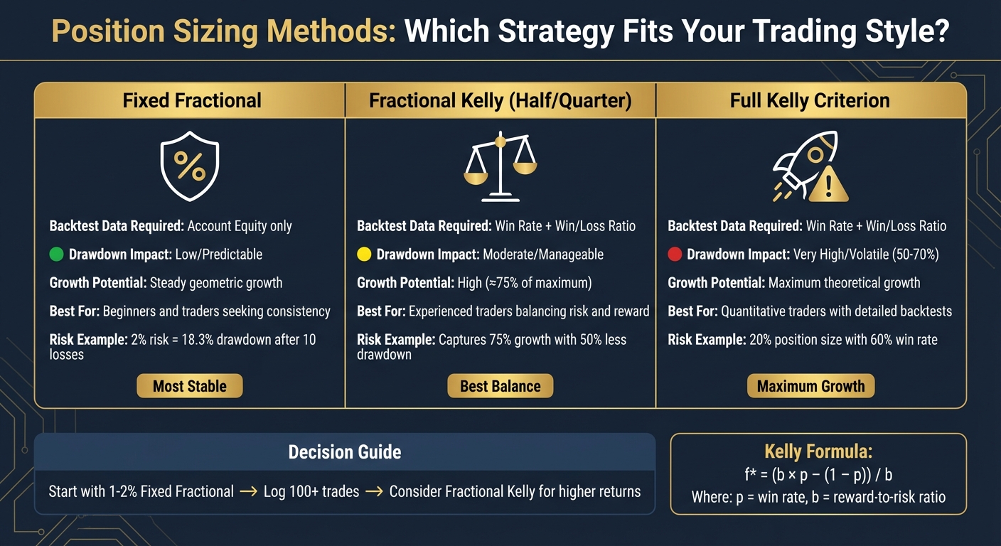
Position Sizing Methods Comparison: Fixed Fractional vs Kelly Criterion
Once you’ve nailed down your strategy’s risk metrics, the next step is tailoring your position sizing to safeguard your capital while aiming for steady growth. By leveraging backtesting data, you can establish clear rules for how much risk to take on each trade. This approach ensures your decisions are grounded in data, not guesswork. Two widely recognized methods for position sizing are the Kelly Criterion and Fixed Fractional Position Sizing – each catering to different levels of risk tolerance and trading experience.
Using the Kelly Criterion for Position Sizing
The Kelly Criterion is a formula-based method that calculates the optimal percentage of your capital to risk on each trade. It uses two key inputs from your backtesting data: the win rate (p) and the reward-to-risk ratio (b). The formula looks like this:
f* = (b × p – (1 – p)) / b
For example, if your backtesting shows a 60% win rate and a 1:1 reward-to-risk ratio, the Kelly Criterion suggests risking 20% of your capital per trade. While this method can maximize long-term growth, it comes with a major downside: during losing streaks, drawdowns can soar to 50–70%.
"A brilliant trading strategy with a genuine edge can still lead to ruin if positions are sized incorrectly." – Michael Brenndoerfer
Because of this risk, most traders opt for Fractional Kelly, which means using only a portion of the calculated Kelly percentage – commonly Half Kelly (50%) or Quarter Kelly (25%). For instance, Half Kelly allows you to capture around 75% of the maximum growth rate while cutting drawdown risk by roughly 50%.
It’s important to note that the Kelly Criterion works best with a large sample size (at least 100 trades) to ensure reliable probabilities. Additionally, you should update your Kelly percentage every 50–100 trades to account for any changes in your strategy’s performance. If the formula gives a negative result, it means the strategy has a negative expectancy, signaling that it’s probably not worth trading.
Fixed Fractional Position Sizing
Fixed Fractional Position Sizing is a simpler and more widely used method, especially among traders at proprietary firms. Here, you risk a fixed percentage of your account equity on every trade – usually between 1% and 2%. This method doesn’t rely on specific backtesting metrics like the Kelly Criterion but instead focuses on consistent risk management.
The formula is straightforward:
Position Size = (Account Equity × Risk %) ÷ Stop Loss Distance
For instance, if you have a $100,000 account and decide to risk 2% ($2,000) with a 10-tick stop-loss, you calculate your position size so that the maximum loss remains $2,000.
One of the standout features of Fixed Fractional Sizing is its self-adjusting nature. During losing streaks, as your account equity decreases, the amount you risk per trade automatically shrinks, which slows down capital erosion. For example:
- A 2% risk model results in an 18.3% drawdown after 10 consecutive losses and a 33% drawdown after 20 losses.
- A 1% risk model, on the other hand, would require over 69 consecutive losses to reach a 50% drawdown.
This method is particularly well-suited for traders aiming for prop firm funding, where consistency and capital preservation take priority. If you’re exploring prop firms, check out reviews on DamnPropFirms, such as their review of Apex Trader Funding at https://damnpropfirms.com/futures-prop-firms/apex-trader-funding/.
Position Sizing Methods Compared
Here’s a quick comparison of the two methods and their trade-offs:
| Method | Backtest Data Required | Drawdown Impact | Growth Potential | Best For |
|---|---|---|---|---|
| Fixed Fractional | Account Equity | Low/Predictable | Steady geometric growth | Beginners and traders seeking consistency |
| Kelly Criterion | Win Rate and Win/Loss Ratio | Very high/volatile | Maximum theoretical growth | Quantitative traders with detailed backtests |
| Fractional Kelly | Win Rate and Win/Loss Ratio | Moderate/manageable | High (≈75% of maximum) | Experienced traders balancing risk and reward |
Fixed Fractional Sizing offers a smoother equity curve and reduces emotional stress during downturns, making it an excellent choice for newer traders or those focused on stability. On the flip side, the Kelly Criterion can deliver maximum growth but requires precise data and the discipline to handle its volatility. Fractional Kelly strikes a middle ground, offering higher growth potential without the extreme risks of Full Kelly.
For most traders, especially those working toward prop firm funding, starting with a 1–2% Fixed Fractional approach is a practical and safe choice. Once you’ve logged over 100 trades and feel confident in your backtesting results, you can explore Fractional Kelly to potentially increase returns while keeping risks manageable.
Setting Stop-Loss and Take-Profit Levels
Once you’ve nailed down your position sizing, the next step is defining clear exit points for both losses and profits. Using static stop-losses – like a flat $500 per contract – can be risky. They don’t adjust to market conditions, which means you might get stopped out during routine price swings in volatile markets or take on too little risk in calmer ones. Instead, dynamic stop-loss and take-profit levels, informed by backtesting, help you adapt to changing conditions. This approach lets you ride winning trades longer while cutting losses early, creating a more balanced risk management strategy.
Using ATR for Dynamic Stop-Loss Adjustments
The Average True Range (ATR) is a handy tool for gauging market volatility. It measures how much a market typically moves over a set period – 14 days is a common choice for futures traders. By multiplying the ATR by a specific factor (known as the multiplier), you can set stop-loss levels that account for normal price fluctuations while still protecting against significant losses.
Here’s the formula:
Stop Loss = Entry Price ± (ATR × Multiplier)
For long positions, subtract the result; for short positions, add it. Backtesting can help fine-tune the multiplier to suit your strategy.
"The Average True Range (ATR) is an indispensable tool that moves the stop-loss order away from being a static barrier and transforms it into a responsive mechanism." – QuantStrategy.io Team
Testing multipliers in small increments (e.g., 1.0x to 5.0x, increasing by 0.25) can reveal the sweet spot for your strategy. For example, backtesting a mean-reversion strategy on the E-mini S&P 500 (ES) from 2017 to 2019 showed that a 1.5x multiplier led to a 45% win rate due to frequent stop-outs. Adjusting to a 2.0x–2.25x multiplier improved the win rate to 58% and boosted the profit factor to 1.7, as stops were placed just beyond typical market noise.
Different markets require different multipliers. For instance:
- E-mini S&P 500 (ES): Tighter stops (around 2.0x ATR) work well due to its structured and liquid nature.
- Crude Oil (CL): Wider stops (3.5x to 4.0x ATR) are better suited to handle geopolitical events and inventory report spikes.
In one five-year backtest for swing trading Crude Oil, a 2.5x multiplier led to drawdowns over 30%. Increasing it to 3.5x–4.0x ATR reduced drawdowns to under 15%.
| Strategy Type | Recommended ATR Multiplier | Market Context |
|---|---|---|
| Scalping / Aggressive Day Trade | 1.5x – 2.0x | Low-noise or range-bound markets |
| Standard Trend Following | 2.5x – 3.0x | Balanced markets with normal pullbacks |
| Swing Trading / Volatile Commodities | 3.5x – 4.5x | High-impact news or geopolitical sensitivity |
For a more advanced approach, consider the Chandelier Exit. This method recalculates the stop-loss based on the highest high (for longs) or lowest low (for shorts) since entry, adjusted by the ATR multiplier. It’s a great way to lock in profits during trends while limiting losses if the market reverses. However, if the ATR stop exceeds your risk tolerance (e.g., 1% of equity), you’ll need to lower your position size or skip the trade.
Testing for Optimal Take-Profit Levels
Dynamic stop-losses are only half the equation – setting effective take-profit levels is just as important. While stop-losses limit your downside, take-profit levels determine how much you capture when the trade goes your way. Backtesting can help you find the best reward-to-risk (R/R) ratio for your strategy. For example:
- A 1:2 R/R ratio means you only need a 34% win rate to break even.
- A 1:3 R/R ratio lowers the breakeven win rate to just 25%.
Testing different R/R ratios (e.g., 1:2, 1:3, 1:5) across a large sample of trades helps identify the most effective setup for your approach.
ATR-based profit targets work similarly to ATR stops, letting you capture larger moves while protecting gains. A common tactic is moving your stop to breakeven after the trade moves favorably by 1 ATR. Then, trail the stop by 2 ATR or 3 ATR to let winners run.
To avoid overfitting, use walk-forward analysis. Optimize your take-profit levels on historical data (the "in-sample" period), then test them on new data (the "out-of-sample" period). Markets evolve, so revisit your multipliers and profit targets every 6–12 months to ensure your strategy stays relevant.
As a general rule, avoid trades with an R/R ratio below 1:1.5. It’s tough to stay profitable below that threshold. If you’re aiming for funding from proprietary trading firms, disciplined take-profit strategies are critical. For more on firms that prioritize solid risk management, check out reviews on DamnPropFirms, like their insights on Take Profit Trader.
Managing Risk Across Multiple Futures Contracts
When trading multiple futures contracts, it might seem like you’re spreading risk. But backtesting often reveals a different story – holding multiple contracts can actually concentrate risk. If your positions tend to move together, you’re effectively making one oversized bet. The trick lies in using backtesting to understand how your positions interact and what happens when markets turn against you. Let’s take a closer look at how correlations affect diversification.
Correlation Analysis for Diversification
Correlation measures how closely two assets move in relation to each other. By analyzing historical price data, you can uncover instances where you’re unintentionally increasing exposure to the same market risks. For example, SPY and QQQ often exhibit a 0.95 correlation, meaning holding both is more like doubling down on one trade rather than achieving true diversification.
This concept highlights your Effective Risk. Imagine you risk 1% on eight trades, each with an 85% correlation – you’re not spreading 8% across independent bets. Instead, you’re exposing yourself to about 6–7% on a single market move. The formula for this is:
Effective Risk = Nominal Risk × √(N × Average Correlation), where N represents the number of positions.
A real-world example is Mark Stevens, who held six tech positions (SPY, QQQ, NVDA, TSLA, AAPL, MSFT) with an average correlation of 82%. This led to a 4.9% effective risk and a $79,000 loss in just one month.
"I lost $79K in ONE MONTH learning CORRELATION RISK is invisible until it kills you. I had 6 ‘diversified’ positions… They were 82% correlated – when one dropped, ALL dropped." – Mark Stevens, Swing Trader
Backtesting also reveals another critical insight: correlations spike during market stress. Assets that typically show low correlation can suddenly align during crises. For instance, during the March 2020 COVID crash, the correlation between Tech and Healthcare sectors surged from 0.25 to 0.92. This means portfolios that seem diversified in calm markets can collapse into a single concentrated risk when volatility strikes.
To manage this, apply the 0.7 Rule: if a new position has a correlation above 0.7 with your existing portfolio, consider skipping the trade or reducing its size. Additionally, when the VIX climbs above 30, assume correlations will trend toward 0.9 and cut position sizes by 50–70%.
Another helpful metric is Effective N, which calculates the true number of independent bets in your portfolio:
Effective N = N / √Avg Correlation. For example, a portfolio of five positions with an average correlation of 0.87 functions as only 1.9 independent bets. This metric ensures you’re not mistaking concentrated risk for diversification.
Simulating Portfolio Drawdowns
Understanding correlations is just one piece of the puzzle. Simulating portfolio drawdowns gives you a clearer picture of your actual risk exposure. Portfolio Heat measures the total dollar risk if all your stops are hit at once. Backtesting can help you set limits that align with your risk tolerance and trading style.
Institutional trading desks often cap portfolio heat at 10–15%, while more conservative retail traders should aim for 3–5%.
Monte Carlo simulations are another powerful tool. These simulations run thousands of "what-if" scenarios, varying volatility and leverage assumptions to provide a range of potential outcomes. For instance, a Monte Carlo analysis of a portfolio with 55% stocks and 45% bonds showed stability at 1.0x leverage, strong performance at 1.5x and 2.0x, but significant stress at 3.0x leverage.
"Monte Carlo simulations let us stress-test portfolios by running thousands of ‘what if’ scenarios with different volatility and leverage assumptions." – Dan Buckley, Chief Analyst, DayTrading.com
Backtesting your portfolio for "What If" scenarios can also reveal vulnerabilities. For example: "If the S&P 500 drops 3% tomorrow, what is the aggregate loss across all futures contracts?". Segmenting your analysis by volatility regimes (e.g., VIX below 20 vs. VIX above 30) can help fine-tune risk parameters for different market conditions.
For traders aiming to secure funding, firms like Apex Trader Funding and Topstep prioritize strong portfolio-level risk management. By backtesting your strategies against their drawdown rules, you can improve your chances of passing evaluations and maintaining funded accounts over time.
Common Mistakes in Using Backtesting Data
Backtesting can offer valuable insights into risk management, but it’s also a common source of costly errors for traders. Spotting these pitfalls early can make a big difference in achieving long-term success.
Overfitting to Historical Data
Overfitting happens when a strategy is overly fine-tuned to historical data, capturing random noise instead of actual market trends. It’s like memorizing answers for a test that doesn’t repeat – great in theory, but it falls apart in real-world trading. In fact, studies show that 78% of published trading strategies fail when applied to data they weren’t optimized for.
A telltale sign of overfitting is an abnormally high Sharpe ratio, especially above 3.0. In live markets, Sharpe ratios over 1.5 are incredibly rare. On average, Sharpe ratios drop by 63% when transitioning from backtesting to live trading.
Take the case of "QuantNewbie87", a Reddit trader who lost $47,000 in 2026. His backtested strategy seemed flawless but failed in live trading because it relied on testing 217 moving average combinations, ignored slippage, and skipped walk-forward analysis. On the flip side, "SystematicTrader42" on QuantConnect managed to keep his live performance within 12% of his backtest by sticking to just three variables: RSI threshold, stop-loss distance, and position sizing.
"If your strategy works too well on past data, it probably doesn’t work at all." – Damon Falk, Expert in International Business
To avoid overfitting, simplify your strategies with just 3 to 5 parameters. Run sensitivity tests by adjusting parameters by 10% to 20%; if the performance collapses, it’s a sign of overfitting. Use walk-forward analysis to improve robustness – it can cut performance decay by 37% compared to random train/test splits. Additionally, pre-registering your trading hypothesis before backtesting can reduce data-snooping bias by 41%.
Now, let’s look at how ignoring shifts in market conditions can derail even a well-tested strategy.
Ignoring Market Regime Changes
Even the best backtested strategies can fail if they don’t account for changes in market conditions. A strategy that thrives in bull markets may falter when volatility spikes or trends reverse. For example, a mean reversion strategy for E-mini S&P 500 (ES) futures showed a 2.5 Profit Factor over 10 years. However, when subjected to walk-forward analysis using 2-year optimization and 6-month test windows, the Profit Factor dropped to 1.3, highlighting its dependence on specific historical conditions.
Market regimes shift constantly. A strategy that performs well in one environment may lose its edge when conditions change. Testing your strategy against historical crisis periods and volatility spikes is crucial. Futures traders, for instance, should analyze data from events like the 2012 drought for agricultural commodities or major VIX spikes to ensure their systems can handle diverse scenarios.
"Backtesting should aim for robustness, not perfection." – Backtestra
This is especially important for traders seeking funding from prop firms like Apex Trader Funding or Take Profit Trader. These firms evaluate strategies across various market conditions, and systems that fail during volatility spikes often violate drawdown rules. To succeed, focus on building strategies that can adapt to changing markets – not just ones that look good in backtests.
Conclusion
Backtesting transforms risk management from mere speculation into a data-driven process. By examining key metrics like maximum drawdown, win rate, and profit factor, traders can fine-tune their position sizing to endure 10–20 consecutive losses without breaching strict prop firm limits. Most evaluation failures stem not from poor strategies but from weak risk management practices.
The real value lies in applying what the data reveals. Strategies like the Fixed Percentage Risk method – risking 0.5%–1% per trade – or the Kelly Criterion can help achieve optimal growth. Using ATR-based dynamic stop-losses (usually set at 1.5–2.0x ATR) ensures your approach adjusts to market volatility. For instance, a strategy with a 1:2 reward-to-risk ratio only requires a 35% win rate to remain profitable. This careful calibration of risk is crucial for developing funding-ready strategies.
These metrics are essential when setting live trading limits or preparing for funding evaluations. For those aiming to secure funded accounts with firms like Apex Trader Funding or Take Profit Trader, understanding your historical maximum drawdown and trailing rules are critical. For example, with a $100,000 account and a 10% drawdown limit, only $10,000 is available for risk. Risking 2% per trade means just five consecutive losses could end your evaluation.
"The point of backtesting isn’t to find a flawless strategy. It’s about deeply understanding how your strategy behaves in different market conditions." – PipBack
Combine these backtesting insights with forward testing to ensure your strategy holds up in today’s markets. Aim to backtest over 5–10 years with 100–200 trades while factoring in real-world costs like commissions and slippage. Paper trading bridges the gap between historical analysis and live trading, helping validate your adjustments under current conditions. This disciplined approach is what separates traders who consistently grow funded accounts from those who struggle to pass evaluations.
FAQs
How do I turn my backtest max drawdown into a real-world risk limit?
To translate your backtest max drawdown into a manageable risk limit for live trading, focus on dynamic position sizing and trailing drawdown adjustments. Here’s how:
- Dynamic Position Sizing: Adjust your position sizes based on your current performance. If you’re approaching your drawdown threshold, scale down your positions to keep potential losses within your acceptable limits.
- Trailing Drawdown: Continuously monitor and adjust your drawdown limit as your account grows. This ensures that your risk remains controlled and aligned with your trading goals.
By combining these strategies, you can effectively manage risk and avoid exceeding your drawdown limits during live trading.
Should I use Fixed Fractional sizing or Fractional Kelly for prop firm rules?
When it comes to prop firm trading rules, Fixed Fractional sizing tends to be the go-to choice. Why? It’s straightforward and fits well within the strict compliance frameworks these firms often enforce. This method involves risking a fixed percentage of your account balance on each trade, making it a safer and more predictable approach for most traders.
On the other hand, the Kelly Criterion is designed to maximize growth mathematically. While it can deliver impressive results, it comes with a catch: it’s far more aggressive. If your win rates or reward-to-risk ratios are even slightly off, the risk increases significantly. For traders who have precise and reliable performance data, Kelly can be a powerful tool for long-term growth. But for the majority, Fixed Fractional sizing offers a more stable and less risky path.
How can I set ATR-based stops without overfitting the multiplier?
When using ATR-based stops, steer clear of rigid or excessively large multipliers that fail to adjust to shifting market conditions. A better approach is to backtest various ATR multiples to find a balance that accounts for volatility without setting stops too narrowly or too broadly. By dynamically tweaking the multiplier to reflect recent market volatility, you can create a more adaptable system that aligns stops with real-time conditions, minimizing the chances of overfitting.